Thursday, August 13, 2009

save a chart to a file format for inclusion in other documents

A chart can be saved in a different file format to be included in other programs by using the copy and paste function. Right click on the chart > copy > paste in another program. You can also use the copy and paste shortcuts when the chart is highlighted use ctrl+c (copy) then ctrl+v (paste) in the other program.

generate and configure charts in a variety of formats

A graph, or a chart as it is known in Excel, is a visual representation of worksheet data. A chart is based on a selection or range of related data. A chart often makes it easier to understand the data in a worksheet because users can easily pick out patterns and trends illustrated in the chart that are otherwise difficult to see.
The quickest and easiest way to create a chart in Excel is to use the Chart Wizard. The Chart Wizard is composed of a series of dialog boxes that give you all the available options for creating a chart.


  1. Choosing the chart type such as pie chart, bar chart, or line chart.

  2. Selecting or verifying the data that will be used to create the chart.

  3. Adding titles to the chart and choosing various chart options such as adding labels and a legend.

  4. Deciding whether to put the chart on the same page as the data or on a separate sheet.

Create a chart in Excel 2007 and in Excel 2003 or change an exisiting chart type in 2003 or 2007 with help from MS online.


display information by using: Filters and Pivot Tables.

The two key tools for filtering and summarizing small data sets are filters and pivot tables. Filters let you see just the items you want, without changing the underlying data. Pivot tables are powerful summary tools, much like statistical software for large databases. PivotTables allow you to create multidimensional data views by dragging and dropping column headings to move data around.
Microsoft online Pivot Tables Tutorial
Filter data in a Pivot Table
Filter data in a range or table

work with data across multiple sheets

To be able to view two or more worksheets at the same time can save a great deal of time.
Microsoft office online can help you understand this:
http://office.microsoft.com/en-us/excel/HP012170431033.aspx?pid=CH100648381033

Sunday, August 9, 2009

configure page layouts

This tutorial by microsoft online explains how page layout view can help fine-tune pages.
http://office.microsoft.com/en-us/excel/HA100215631033.aspx?pid=CH100798591033

manipulate page breaks
microsoft online should be able to help with this.

sort selected areas of the spreadsheet

Sorting data is one of the basics of spreadsheet usage, once it is structured it will be greatly easier to work with. This tutorial will help sort selected areas of the spreadsheet. http://www.ofzenandcomputing.com/zanswers/314

and to an extent this tutorial explains "how to sort data in a range or table"

interchange information with other applications

The most effective way to interchange information with Excel is to use the copy and paste functions. For example to bring data into Access from Excel, you can copy data from an Excel worksheet and paste it into an Access datasheet, import an Excel worksheet into an Access table, or link to an Excel worksheet from an Access table.

This microsoft office online tutorial will help explain how to interchange information from Excel.
http://office.microsoft.com/en-us/excel/HA100963001033.aspx?pid=CH100648471033

record and run macro routines to automate processing

A macro automates a complex task. Excel macros can perform complicated series of actions or simply record commonly used commands.


This video will help explain how to record a macro.
http://h30187.www3.hp.com/tutorials/viewHowTo/p/courseId/14169/Microsoft_Excel_2007.htm?courseSessionId=83396&campusId=10129&webPageId=1000017

How to run a macro
This tutorial by microsoft will help explain how to run a macro. http://office.microsoft.com/en-us/excel/HP100141131033.aspx?pid=CH101001571033

Change the format of a cell

  • text size - text size can be formatted by using the format cells toolbar located above the workspace.
  • or can also be formatted by pressing (ctrl + shift + F) to bring up the format cells dialogbox.


  • For numbers that are already entered on a worksheet, you can increase or decrease the number of places that are displayed after the decimal point by using the Increase Decimal and Decrease Decimal buttons.

Thursday, August 6, 2009

manipulate rows and columns of a spreadsheet and apply a variety of formats

Set a column to a specific width

  1. Select the column or columns that you want to change.

  2. On the Home tab, in the Cells group, click Format.

    Excel Ribbon Image

  3. Under Cell Size, click Column Width.
  4. In the Column width box, type the value that you want.

Change the column width to automatically fit the contents (auto fit)

  1. Select the column or columns that you want to change.
  2. On the Home tab, in the Cells group, click Format.

    Excel Ribbon Image

  3. Under Cell Size, click AutoFit Column Width.

Tip To quickly autofit all columns on the worksheet, click the Select All button and then double-click any boundary between two column headings.

Select All button


Match the column width to another column

  1. Select a cell in the column that has the width that you want to use.
  2. On the Home tab, in the Clipboard group, click Copy, and then select the target column.

    Excel Ribbon Image

  3. On the Home tab, in the Clipboard group, click the arrow below Paste, and then click Paste Special.
  4. Under Paste, select Column widths.


Change the default width for all columns on a worksheet or workbook

The value for the default column width indicates the average number of characters of the standard font that fit in a cell. You can specify a different number for the default column width for a worksheet or workbook.

  1. Do one of the following:
    • To change the default column width for a worksheet, click its sheet tab.
    • To change the default column width for the entire workbook, right-click a sheet tab, and then click Select All Sheets on the shortcut menu (shortcut menu: A menu that shows a list of commands relevant to a particular item. To display a shortcut menu, right-click an item or press SHIFT+F10.).

    Excel sheet tabs

  2. On the Home tab, in the Cells group, click Format.

    Excel Ribbon Image

  3. Under Cell Size, click Default Width.
  4. In the Default column width box, type a new measurement.

Tip If you want to define the default column width for all new workbooks and worksheets, you can create a workbook template or a worksheet template, and then base new workbooks or worksheets on those templates.


Change the width of columns by using the mouse

Do one of the following:

  • To change the width of one column, drag the boundary on the right side of the column heading until the column is the width that you want.

    Column boundary being dragged

  • To change the width of multiple columns, select the columns that you want to change, and then drag a boundary to the right of a selected column heading.
  • To change the width of columns to fit the contents, select the column or columns that you want to change, and then double-click the boundary to the right of a selected column heading.
  • To change the width of all columns on the worksheet, click the Select All button, and then drag the boundary of any column heading.

    Select All button

Set a row to a specific height

  1. Select the row or rows that you want to change.
  2. On the Home tab, in the Cells group, click Format.

    Excel Ribbon Image

  3. Under Cell Size, click Row Height.
  4. In the Row height box, type the value that you want.

Change the row height to fit the contents

  1. Select the row or rows that you want to change.
  2. On the Home tab, in the Cells group, click Format.

    Excel Ribbon Image

  3. Under Cell Size, click AutoFit Row Height.

Tip To quickly autofit all rows on the worksheet, click the Select All button and then double-click the boundary below one of the row headings.

Select All button

Change the height of rows by using the mouse

Do one of the following:

  • To change the row height of one row, drag the boundary below the row heading until the row is the height that you want.

    Row boundary being dragged

  • To change the row height of multiple rows, select the rows that you want to change, and then drag the boundary below one of the selected row headings.
  • To change the row height for all rows on the worksheet, click the Select All button, and then drag the boundary below any row heading.

    Select All button

  • To change the row height to fit the contents, double-click the boundary below the row heading.


Rearrange (transpose) data from columns to rows or vice versa

If data is entered in columns or rows, but you want to rearrange that data into rows or columns instead, you can quickly transpose the data from one to the other.

For example, the regional sales data that is organized in columns appears in rows after transposing the data, as shown in the following graphics.

Regional data in columns

Regional data in rows

  1. On the worksheet, do the following:
    • To rearrange data from columns to rows, select the cells in the columns that contain the data.
    • To rearrange data from rows to columns, select the cells in the rows that contain the data.
  2. On the Home tab, in the Clipboard group, click Copy Button image.

    Clipboard group on Excel Ribbon

    Keyboard shortcut To copy the selected data, you can also press CTRL+C.

    Note You can only use the Copy command to rearrange the data. To complete this procedure successfully, do not use the Cut Button image command.

  3. On the worksheet, select the first cell of the destination rows or columns into which you want to rearrange the copied data.

    Note Copy areas (copy area: The cells that you copy when you want to paste data into another location. After you copy cells, a moving border appears around them to indicate that they've been copied.) and paste areas (paste area: The target destination for data that's been cut or copied by using the Office Clipboard.) cannot overlap. Make sure that you select a cell in a paste area that falls outside of the area from which you copied the data.

  4. On the Home tab, in the Clipboard group, click the arrow below Paste, and then click Transpose.
  5. After the data is transposed successfully, you can delete the data in the copy area.

Tip If the cells that you transpose contain formulas, the formulas are transposed and cell references to data in transposed cells are automatically adjusted. To make sure that formulas continue to refer correctly to data in nontransposed cells, use absolute references in the formulas before you transpose them.

This video may help with understanding how to format rows and columns: video

http://office.microsoft.com/en-gb/excel/HP012163831033.aspx?pid=CH100648141033

http://office.microsoft.com/en-gb/excel/HP102245021033.aspx?pid=CH100648341033

export spreadsheet data in a variety of formats

After you have imported XML data, mapped the data to cells in your worksheet, and made changes to the data, you often want to export or save the data to an XML file. There are two ways to export XML data from a Microsoft Office Excel 2007 worksheet:

  • Microsoft Office Help Online recommends using the Export command in the XML group on the Developer tab to get XML data out of your worksheet.
  • For backward compatibility with earlier XML functionality, you can still use the Other Formats command on the Save As submenu of the Microsoft Office Button Button image.

Export XML data in mapped cells to an XML data file

  1. If the Developer tab is not available, do the following to display it:
    1. Click the Microsoft Office Button Button image, and then click Excel Options.
    2. In the Popular category, under Top options for working with Excel, select the Show Developer tab in the Ribbon check box, and then click OK.

      Note The Ribbon is a component of the Microsoft Office Fluent user interface.

  2. On the Developer tab, in the XML group, click Export.

    XML group in Ribbon

    Note If a small Export XML dialog box appears, click the XML map that you want to use, and then click OK.

    The Export XML dialog box will only appear if an XML table is not selected and if the workbook contains more than one XML map.

  3. In the large Export XML dialog box, in the File name box, type a name for the XML data file.
  4. Click Export.

Note There may be headings or labels in your worksheet that are different from the XML element names in the XML map. However, the XML element names are always used when you export or save XML data from the worksheet.

http://office.microsoft.com/en-gb/excel/HP102064011033.aspx?pid=CH100648521033 - Will explain XML data in greater detail


import data from a variety of sources

The main benefit of connecting to external data is that you can periodically analyze this data in Microsoft Office Excel without repeatedly copying the data, which is an operation that can be time-consuming and error-prone. After connecting to external data, you can also automatically refresh (or update) your Excel workbooks from the original data source whenever the data source is updated with new information.

Important Connections to external data may be disabled on your computer. To connect to data when you open a workbook, you must enable data connections by using the Trust Center bar, or by putting the workbook in a trusted location. For more information, see Create, remove, or change a trusted location for your files, Add, remove, or view a trusted publisher, and View my security settings in the Trust Center.

  1. On the Data tab, in the Get External Data group, click Existing Connections.

    Excel Ribbon Image

  2. In the Existing Connections dialog box, in the Show drop-down list, do one of the following:
    • To display all connections, click All Connections. This is selected by default.
    • To display only the recently used list of connections, click Connections in this Workbook.

      This list is created from connections that you have already defined, that you have created by using the Select Data Source dialog box of the Data Connection Wizard, or that you have previously selected as a connection from this dialog box.

    • To display only the connections that are available on your computer, click Connection files on this computer.

      This list is created from the My Data Sources folder that is usually stored in the My Documents folder.

    • To display only the connections that are available from a connection file that is accessible from the network, click Connection files on the Network.

      This list is created from an Excel Services Data Connection Library (DCL) on a Microsoft Office SharePoint Server 2007 site. A DCL is a document library in a Microsoft Office SharePoint Services 2007 site that contains a collection of Office Data Connection (ODC) files (.odc). Typically, a DCL is set up by a site administrator, who can also configure the SharePoint site to display ODC files from this DCL in the External Connections dialog box. For more information, see Office SharePoint Server 2007 Central Administration Help.

    • Tip If you do not see the connection that you want, you can create a connection. Click Browse for More, and then in the Select Data Source dialog box, click New Source to start the Data Connection Wizard so that you can select the data source that you want to connect to.

    Note If you choose a connection from the Connection files on the network or Connection files on this computer categories, the connection file is copied into the workbook as a new workbook connection, and then it is used as the new connection information.

  3. Select the connection that you want, and then click Open.
  4. In the Import Data dialog box, under Select how you want to view this data in your workbook do one of the following:

    Important The Select how you want to view this data in your workbook section and its options, as shown in the following list, are not available for text, Web Query, and XML data connections. If you are connecting to such data, continue to step 5.

    • To create a table for simple sorting and filtering, click Table.
    • To create a PivotTable report for summarizing large amounts of data by aggregating and subtotaling the data, click PivotTable Report.
    • To create a PivotTable report, and PivotChart report for visually summarizing data, click PivotChart and PivotTable Report.
    • To store the selected connection in the workbook for later use, click Only Create Connection.

      Use the Only Create Connection option to store the selected connection in the workbook for later use. For example, if you are connecting to an Online Analytical Processing (OLAP) cube data source and you intend to convert PivotTable cells to worksheet formulas by using the Convert to Formulas command (On the Options tab, in the Tools group, click OLAP tools), you can use this option because you don't need to save the PivotTable report.

  5. Under Where do you want to put the data?, do one of the following:
    • To place the PivotTable or PivotChart report in an existing worksheet, select Existing worksheet, and then type the first cell in the range of cells where you want to locate the PivotTable report.

      Alternatively, click Collapse Dialog Button image to temporarily hide the dialog box, select the beginning cell on the worksheet, and then press Expand Dialog Button image.

  6. To place the PivotTable report in a new worksheet starting at cell A1, click New worksheet.
  7. Optionally, you can change connection properties by clicking Properties, by making your changes in the Connection Properties , External Data Range , or XML Map Properties dialog boxes, and then by clicking OK.
http://office.microsoft.com/en-gb/excel/HP100898981033.aspx?pid=CH100648471033

print all or selected parts of a spreadsheet

Print an Excel table

If the data that you want to print is in a Microsoft Office Excel table, you can print just the Excel table.

  1. Click a cell within the table to activate the table.
  2. Click Microsoft Office Button Button image, and then click Print.

    Keyboard shortcut You can also press CTRL+P.

  3. Under Print what, click Table.

Define or clear a print area on a worksheet
If you print a specific selection on the worksheet frequently, you can define a print area (print area: One or more ranges of cells that you designate to print when you don't want to print the entire worksheet. If a worksheet includes a print area, only the print area is printed.) that includes just that selection. When you print the worksheet after defining a print area, only the print area will print. You can add cells to expand the print area as needed, and you can clear the print area to print the entire worksheet again.

Set a print area

  1. On the worksheet, select the cells that you want to define as the print area.
  2. On the Page Layout tab, in the Page Setup group, click Print Area, and then click Set Print Area.

Note The print area that you set is saved when you save the workbook.

Add cells to an existing print area

  1. On the worksheet, select the cells that you want to add to the existing print area.
  2. On the Page Layout tab, in the Page Setup group, click Print Area, and then click Add to Print Area.

Clear a print area

  1. Click anywhere on the worksheet for which you want to clear the print area.
  2. On the Page Layout tab, in the Page Setup group, click Clear Print Area.

recalculate values after editing a cell

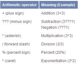
To use formulas efficiently, there are three important considerations you need to understand:

Calculation is the process of computing formulas and then displaying the results as values in the cells that contain the formulas. To avoid unnecessary calculations, Microsoft Office Excel automatically recalculates formulas only when the cells that the formula depends on have changed. This is the default behavior when you first open a workbook and when you are editing a workbook. However, you can control when and how Excel recalculates formulas.

Iteration is the repeated recalculation of a worksheet until a specific numeric condition is met. Excel cannot automatically calculate a formula that refers to the cell — either directly or indirectly — that contains the formula. This is called a circular reference. If a formula refers back to one of its own cells, you must determine how many times the formula should recalculate. Circular references can iterate indefinitely. However, you can control the the maximum number of iterations and the amount of acceptable change.

Precision is a measure of the degree of accuracy for a calculation. Excel stores and calculates with 15 significant digits of precision. However, you can change the precision of calculations so that Excel uses the displayed value instead of the stored value when it recalculates formulas.

Replace a formula with its result

You can convert the contents of a cell that contains a formula so that the calculated value replaces the formula. If you want to freeze only part of a formula, you can replace only the part you don't want to recalculate. Replacing a formula with its result can be helpful if there are many or complex formulas in the workbook and you want to improve performance by creating static data.

You can convert formulas to their values on either a cell-by-cell basis or convert an entire range at once.

Important Make sure you examine the impact of replacing a formula with its results, especially if the formulas reference other cells that contain formulas. It's a good idea to make a copy of the workbook before replacing a formula with its results.

Replace formulas with their calculated values

Caution When you replace formulas with their values, Microsoft Office Excel permanently removes the formulas. If you accidentally replace a formula with a value and want to restore the formula, click Undo Button image immediately after you enter or paste the value.

  1. Select the cell or range of cells that contains the formulas.

    If the formula is an array formula (array formula: A formula that performs multiple calculations on one or more sets of values, and then returns either a single result or multiple results. Array formulas are enclosed between braces { } and are entered by pressing CTRL+SHIFT+ENTER.), select the range that contains the array formula.

    ShowHow to select a range that contains the array formula

    1. Click a cell in the array formula.
    2. On the Home tab, in the Editing group, click Find & Select, and then click Go To.
    3. Click Special.
    4. Click Current array.
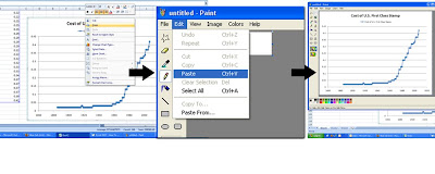
  2. Click Copy Button image.
  3. Click Paste Button image .
  4. Click the arrow next to Paste Options Button image, and then click Values Only.

The following example shows a formula in cell D2 that multiplies cells A2, B2, and a discount derived from C2 to calculate an invoice amount for a sale. To copy the actual value instead of the formula from the cell to another worksheet or workbook, you can convert the formula in its cell to its value by doing the following:

  1. Press F2 to edit the cell.
  2. Press F9, and then press ENTER.

    The formula is shown in the formula bar

    After you convert the cell from a formula to a value, the value appears as 1932.322 in the formula bar. Note that 1932.322 is the actual calculated value, and 1932.32 is the value displayed in the cell in a currency format.

    The value is shown in the formula bar

    Tip When you are editing a cell that contains a formula, you can press F9 to permanently replace the formula with its calculated value.

Replace part of a formula with its calculated value

There may be times when you want to replace only a part of a formula with its calculated value. For example, you want to lock in the value that is used as a down payment for a car loan. That down payment was calculated based on a percentage of the borrower's annual income. For the time being, that income amount won't change, so you want to lock the down payment in a formula that calculates a payment based on various loan amounts.

Caution When you replace a part of a formula with its value, that part of the formula cannot be restored.

  1. Click the cell that contains the formula.
  2. In the formula bar (formula bar: A bar at the top of the Excel window that you use to enter or edit values or formulas in cells or charts. Displays the constant value or formula stored in the active cell.) Formula bar, select the portion of the formula that you want to replace with its calculated value. When you select the part of the formula that you want to replace, make sure that you include the entire operand (operand: Items on either side of an operator in a formula. In Excel, operands can be values, cell references, names, labels, and functions.). For example, if you select a function, you must select the entire function name, the opening parenthesis, the arguments (argument: The values that a function uses to perform operations or calculations. The type of argument a function uses is specific to the function. Common arguments that are used within functions include numbers, text, cell references, and names.), and the closing parenthesis.
  3. To calculate the selected portion, press F9.
  4. To replace the selected portion of the formula with its calculated value, press ENTER.

    If the formula is an array formula (array formula: A formula that performs multiple calculations on one or more sets of values, and then returns either a single result or multiple results. Array formulas are enclosed between braces { } and are entered by pressing CTRL+SHIFT+ENTER.), press CTRL+SHIFT+ENTER.

http://office.microsoft.com/en-gb/excel/HP100541491033.aspx

http://office.microsoft.com/en-gb/excel/HP100662581033.aspx?pid=CH100648421033#Replace%20a%20formula%20with%20its%20calculated%20value

Comparison Operators

You can compare two values with the following operators. When two values are compared by using these operators, the result is a logical value either TRUE or FALSE.

http://office.microsoft.com/en-gb/excel/HP100788861033.aspx?pid=CH100648411033


use built-in functions with a minimum set providing the equivalent of

Arithmetic:
SUM, MAXIMUM, MINIMUM, COUNT, ABSOLUTE VALUE, SQUARE ROOT, INTEGER PART
Statistical:
MEAN, STANDARD DEVIATION
Logical:
IF (allows selection of a value on the basis of a simple relation being TRUE or FALSE)
Other:
LOOKUP

Wednesday, August 5, 2009

enter formulas into cells to calculate values

To perform basic mathematical operations such as addition, subtraction, or multiplication; combine numbers; and produce numeric results, use the following arithmetic operators.
Examples of these arithmetic operators were seen in the previous post "use arithmetic operators to create formulas"


The link listed below is a useful tutorial on how to use excel as a simple arithmetic calculator by producing formulas and entering them into cells to calculate values
http://phoenix.phys.clemson.edu/tutorials/excel/arithmetic.html

use arithmic operators to create formulas

To perform basic mathematical operations such as addition, subtraction, or multiplication; combine numbers; and produce numeric results, use the following arithmetic operators which are shown in the table below


1. Decide what your formula needs to calculate. Do you need to add up a column or row of figures? Do you need to divide one cell's value by another cell's value?
2. Start with an “=” (equal sign). Every formula will start with an equal sign. If you don't begin with this symbol, your formula will not work.
3. Put the first cell's name next. Each cell has a name assigned to it. “A1” is the first cell in the worksheet. Find the cell name by looking at the row and column that it is in.
4. Use the correct function key: “*” for multiplication, “/” for division, “+” is for addition and “-“ for subtraction.
5. Insert the last cell name. This is just like a math problem. Use the same rules as a simple math problem and your formula will work for you.
6. Hit “Enter.” Does your formula work? Double-check to make sure the components of the formula are correct.


http://office.microsoft.com/en-us/excel/HP051986971033.aspx

Tuesday, August 4, 2009

copy (replicate) cells using both absolute and relative referencing

Relative Cell References

This is the most widely used type of cell reference in formulas. Relative cell references are basic cell references that adjust and change when copied or when using AutoFill. In more simple terms, the cells are adjusted using the same formula from the previous cell references to the other cells intended to be adjusted and changed according with the formula.

Example:
=SUM(B5:B8), as shown below, changes to =SUM(C5:C8) when copied across to the next cell.


Absolute Cell References
Situations arise in which the cell reference must remain the same when copied or when using AutoFill. Dollar signs are used to hold a column and/or row reference constant.

Example:
In the example below, when calculating commissions for sales staff, you would not want cell B10 to change when copying the formula down. You want both the column and the row to remain the same to refer to that exact cell. By using $B$10 in the formula, neither changes when copied.


http://web.pdx.edu/~stipakb/CellRefs.htm

enter text, numeric values and formulas into cells

  • Text that is typed will always appear in the active cell the same will happen for numeric values and formulas (which will calculate by hitting enter). More simply when you click a cell, the text, numeric values and formulas you type will appear in this cell.
  • Click the cell where you want the text to appear. The bold border moves to this cell, showing that it is the active cell.

  • Type the text. What you type appears in the active cell and in the formula bar. If you make a mistake while typing, press Backspace and correct it.
    When you have completed the contents for one cell, press Enter.